Rapid Detailed Comparison of Polymer Samples by T-Wave Ion Mobility

In this application note, SYNAPT G2-S HDMS can be used as a “fingerprint” to rapidly characterize polymer samples. When ion mobility is coupled with mass spectrometry, an additional mode of separation can be achieved that is capable of differentiating ions according to their shape, size, mass-to-charge ratio, and charge state. This means minor changes in a synthetic polymer are more likely to be identified.

Benefits

• Rapid data collection
• Polymer “fingerprinting”
• Polymer backbone architecture confirmation

Polymers are typically very complex materials, requiring several analytical techniques to fully characterize them. Since the introduction of softer ionization techniques, Electrospray Ionization and Matrix Assisted Laser Desorption Ionization, mass spectrometry has increasingly been adopted by the industry to provide additional and complementary information about a sample.

Mass spectrometry can be used to identify many features of a polymer, including end groups, molecular weight distribution, backbone architecture, and repeat unit chemistry. Confirming the chemistry and architecture of a polymer is important because it has a direct impact on its physical properties, for example, density, strength, viscosity, and glass transition temperature. The physical properties of a polymer affect the industrial application that it can be used for.

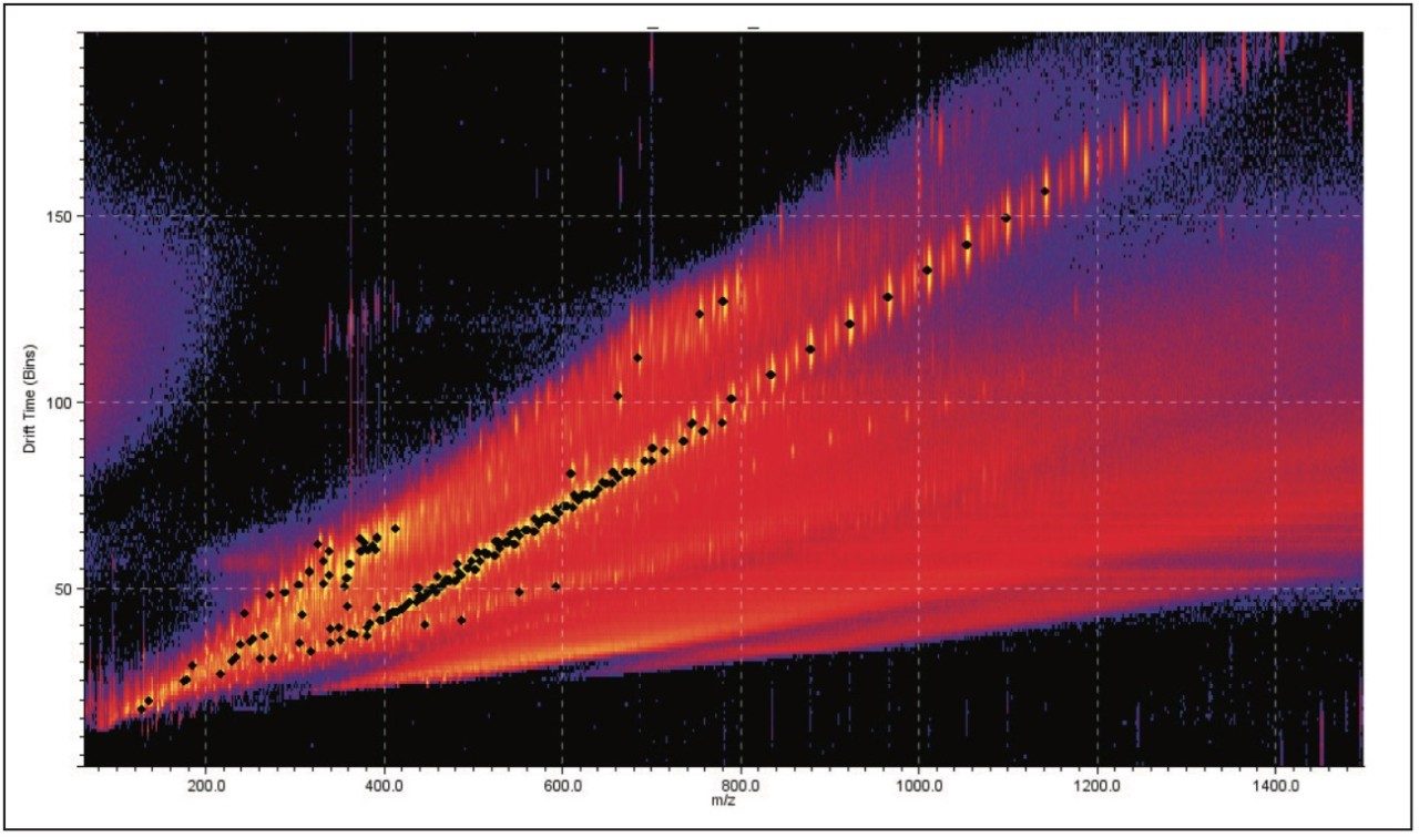
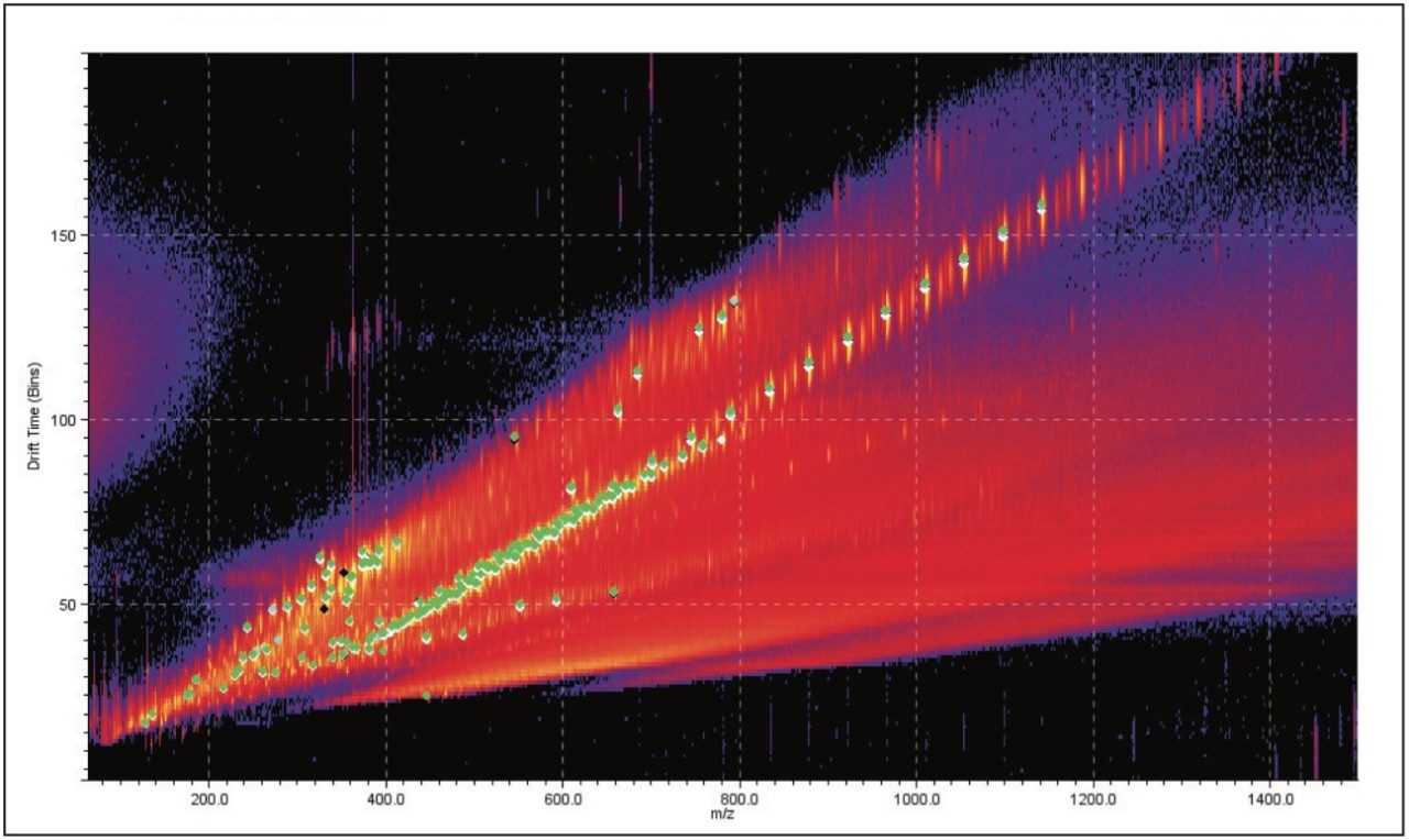
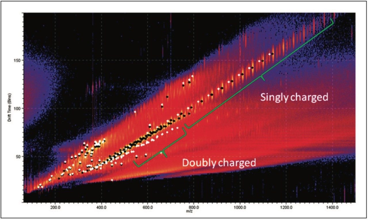
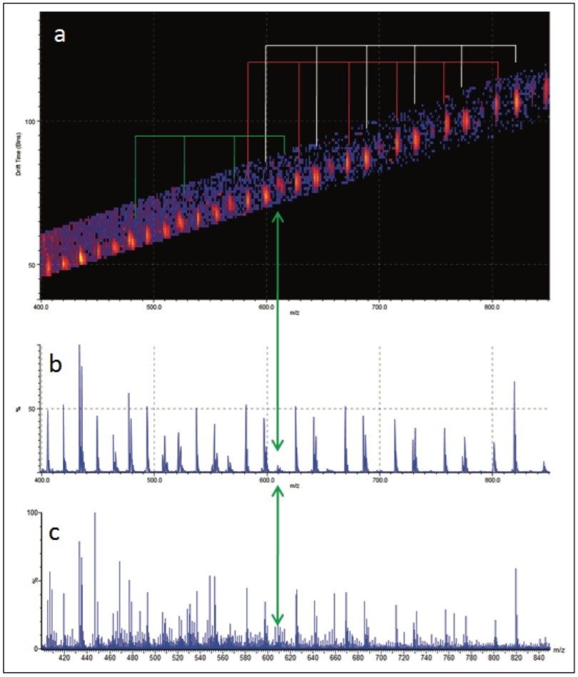
These industrial applications are becoming increasingly sophisticated, demanding increasingly complex chemistries and as a consequence more advanced analyticaltechniques. When ion mobility is coupled with mass spectrometry, an additional mode of separation can be achieved that is capable of differentiating ions according to their shape, size, mass-to-charge ratio, and charge state. This means minor changes in a synthetic polymer are more likely to be identified.

The mobility plots generated by T-Wave ion mobility separations and mass spectrometry can be used as a “fingerprint” to rapidly characterize a sample.¹ This application note demonstrates how data can be collected, samples compared, and tools to help identify any difference.

Sample preparation

The polyethylene glycol (PEG) samples were first dissolved in 50:50 acetonitrile:water before further dilution and the addition of sodium iodide to produce the following:

250 ppb characterized PEG 1000 and 25 ppb sodium iodide

250 ppb uncharacterized PEG and 25 ppb sodium iodide.

A fully characterized linear PEG 1000 sample (structure shown in Figure 1) was infused into the Waters SYNAPT G2-S at 10 μL/min. Figure 2 is a mobility plot generated by DriftScope Software. It shows mass-to-charge ratio on the X-axis, drift time on the Y-axis, and ion intensity is represented by color. The data show a series of ions running diagonally across the mobility plot. The drift time of an ion is determined by a number of factors including size, shape, and charge,² typically referred to as a collision cross section (CCS) measurement and reported in Ų. The larger the ion, the longer it will take to drift through the ion mobility cell.²

DriftScope has a peak detection function, which will identify ions above a selected threshold. These ions have been identified with a black spot in Figure 2.

The 3D size of a polymeric ion is governed by several factors: the monomer units, their 3D arrangement, the backbone connectivity, and the cation(s)³. Therefore, when drift time, ion intensity, and exact mass measurements are combined, the resulting mobility plots are distinctive and could be considered as a “fingerprint” for a polymer sample.

DriftScope Software allows users to export peak detection lists and overlay the results from different samples. Figure 3 shows five samples overlaid. We can see that the data points sit in the same place. This means that the exact mass, ion intensity, and collision cross section area are consistent from sample to sample.

Figure 4 is a comparison between the fully characterized linear PEG sample and an uncharacterized PEG sample. The uncharacterized sample showed a similar ion distribution of singly and doubly charged ions, with a mass difference of 44 Da, consistent with the ethylene glycol repeat unit. A very quick visual inspection of the mobility plot revealed significant differences. The singly charged ion series had slightly different masses but the drift time of the ions are closely related, therefore their 3D size must be similar. 

The doubly charged ion series is the region of most difference between the samples. The most interestingobservation about these ions is the drift time. The uncharacterized sample had a much shorter drift time for ions with acomparable m/z value. This tells us the doubly charged ions in the uncharacterized sample must be more compact.

To gain more information about the samples MS/MS experiments were performed. Precursor ions where chosen with the minimum difference in m/z, to make the results as comparable as possible. Figure 5 shows the two MS/MS spectra; in both spectra ion series were observed with a mass difference of 44 Da. This confirmed the presence of ethylene glycol repeat units in both samples. The most interesting difference in the results was not the change in mass of the ions generated but the pattern. This indicates that the difference between the two PEG samples was not the backbone architecture but with the different end groups. To confidently interpret the MS/MS spectrum it is important to understand the fragmentation mechanism of the polymer.

Figure 6 shows an annotated MS/MS spectrum of the fully characterized linear PEG sample. Two series of ions have been labeled, both series have a 44 mass unit difference. Due to the symmetry of the molecule both fragmentation pathways can happen at either end of the polymer. The proposed fragmentation pathways for each series of ions are shown in Figure 7.

The MS/MS spectrum of the uncharacterized sample is far more complicated. There are several series of ions with a mass difference of 44 Da. The associated mobility plot has a main series of ions running across from the top right-hand side to the bottom left-hand side. This is an ideal place to start interpreting the data. Figure 8 shows the results of a data selection within DriftScope. Two series of ions have been identified with red or white lines in the mobility plot. At 608 m/z a third series of ions became clearly visible, labeled with the green arrow and lines. This series of ions was easy to identify in the mobility plot and extracted mass spectrum. Figure 8c shows the full mass spectrum and demonstrates how difficult it would have been to identify this third ion series without T-Wave ion mobility and mass spectrometry.

The linear PEG sample does not contain an equivalent third series of ions. A mass of 608 m/z is consistent with the loss of three end groups, four ethylene glycol repeat units, and a fragmentation within the fifth ethylene glycol repeat unit. This would suggest that the unknown sample is branched rather than linear because it is not possible for a linear polymer to have three end groups.

Samples were simply dissolved and a cationizing agent added, before infusing directly into the SYNAPT G2-S for just five minutes. Differences between the samples were identified by visual inspection of the mobility plot, followed by more detailed MS/MS analysis. Interpretation of the MS/MS results indicated the uncharacterized sample was branched rather than linear. The ion series that allowed this conclusion to be drawn was clearly visible in the mobility plot but not in the traditional mass spectrum.

A polymer’s physical properties can be affected by the backbone architecture, and as a consequence the industrial applications it can be used for. The ability to confirm the connectivity of a polymer is a vital part of research and development, as well as quality control in a manufacturing environment.

1. S Trimpin, DE Clemmer. Anal Chem. (2008) 80: 9073-9083.
2. An Introduction to Waters T-Wave Devices, Unique Technology for Advanced MS Capabilities. Waters white paper. no. 7200004177en. April, 2012.
3. J Hoskins, S Trimpin, S Grayson. Macromolecules. (2011) 44: 6915.