Impact of Detector Settings on the Plate Count Calculation for 1.7 µm Particle Columns

The purpose of this application note is to show the effect of the detector settings on the measured efficiency of 1.7 μm particle columns.

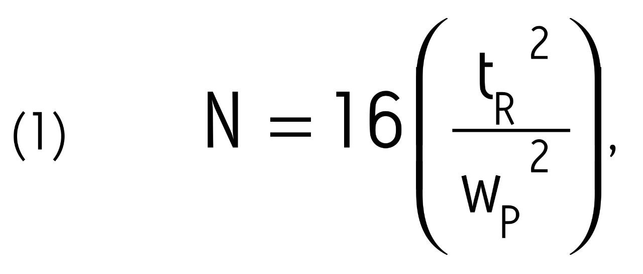
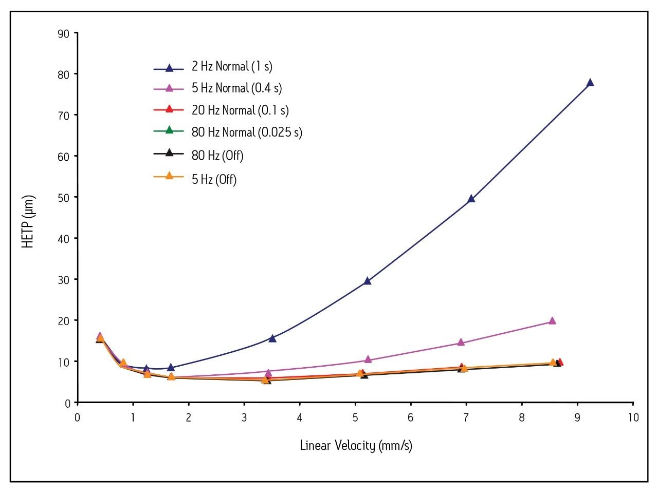
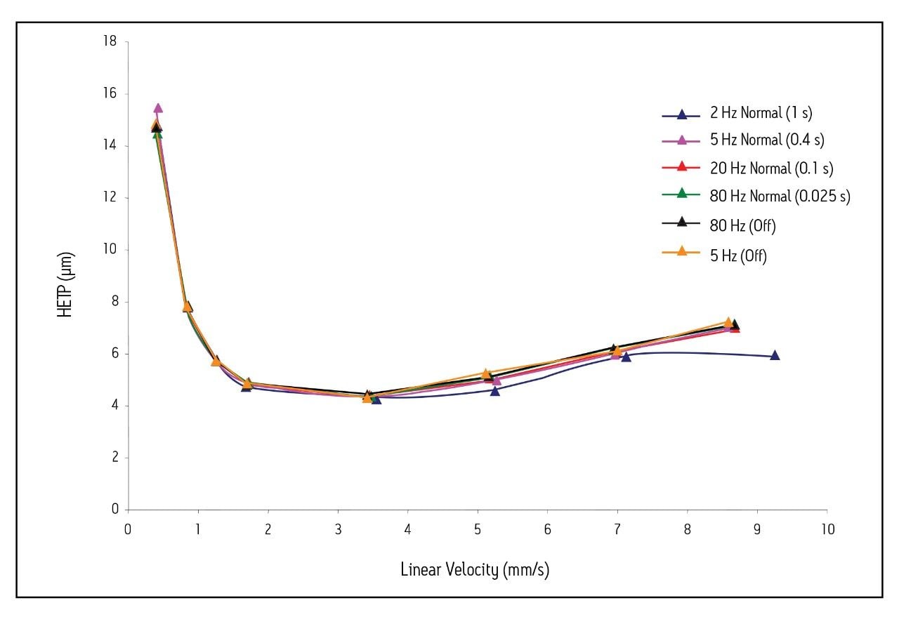
There are several mathematical equations that can be used to determine HPLC column efficiency based on experimental data [1]. One of the most popular of these equations is the van Deemter equation, which plots linear velocity (flow rate) on the x-axis and the height equivalent to a theoretical plate (HETP) on the y-axis [2]. From this plot, one can obtain the flow rate at which the column gives the greatest resolving power for a particular analyte. As column packing particle size decreases, this optimum flow rate increases, and the increase of HETP with linear velocity is less dramatic. Thus, smaller particle columns can be operated at faster flow rates with minimal compromise in performance. This is the basis of UPLC technology.

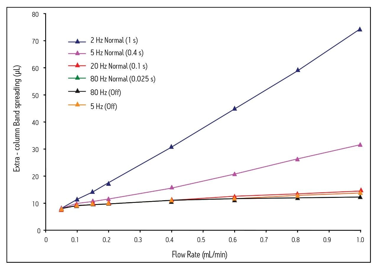
However, narrowbore (2.1 mm i.d.) columns packed with smaller particles are more susceptible to extra-column band spreading than larger diameter columns [3]. Extra-column band spreading is the undesirable widening of a chromatographic peak caused by the LC system. There are two sources of extra-column band spreading. The first one is volumetric in nature and occurs in the system tubing and fittings, column frits, injector, and detector flow cell. The second contribution stems from time-related events such as the sampling rate and/or the detector time constant, which is a time-window based filtering that reduces peak-to-peak noise in order to improve sensitivity.

Previous work has proven that accurate calculation of column efficiency for 1.7 μm particle columns requires an LC instrument with minimal extra-column band spreading and the ability to operate at elevated pressure [3]. It also requires that this instrumentation be used properly to ensure that the resolving power produced by 1.7 μm particle columns is preserved all the way through the detection process.

One aspect of this is reducing extra-column effects by minimizing tubing length and diameter. Another aspect is using the appropriate detector settings, which can also have a significant impact on the perceived system band spreading and column efficiency. In many published reports, the detector settings used to determine column plate count are not optimized, or simply not reported. Under these circumstances, the actual column performance can be misrepresented, typically in an unfavorable manner [4].

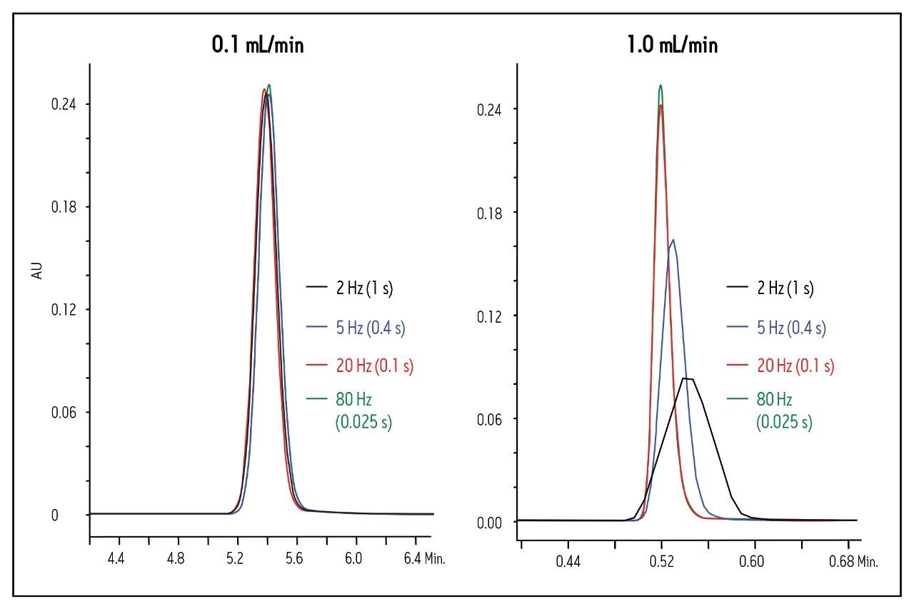
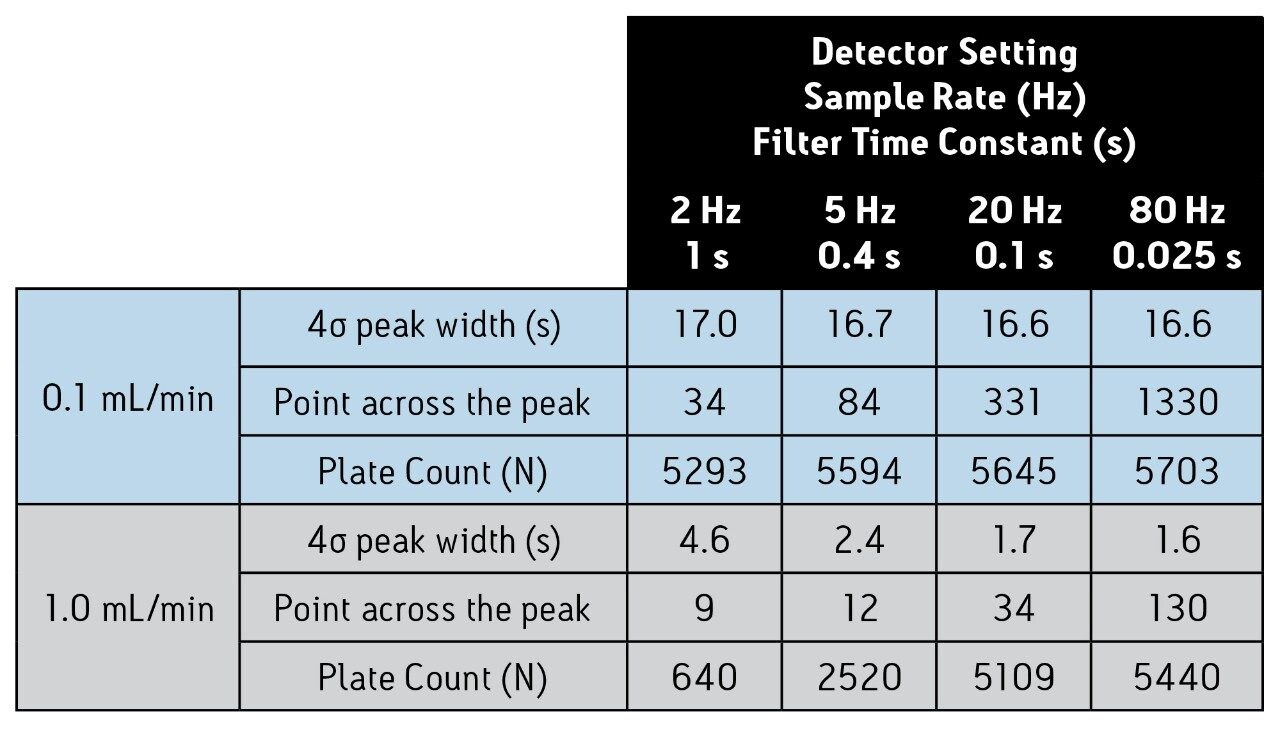
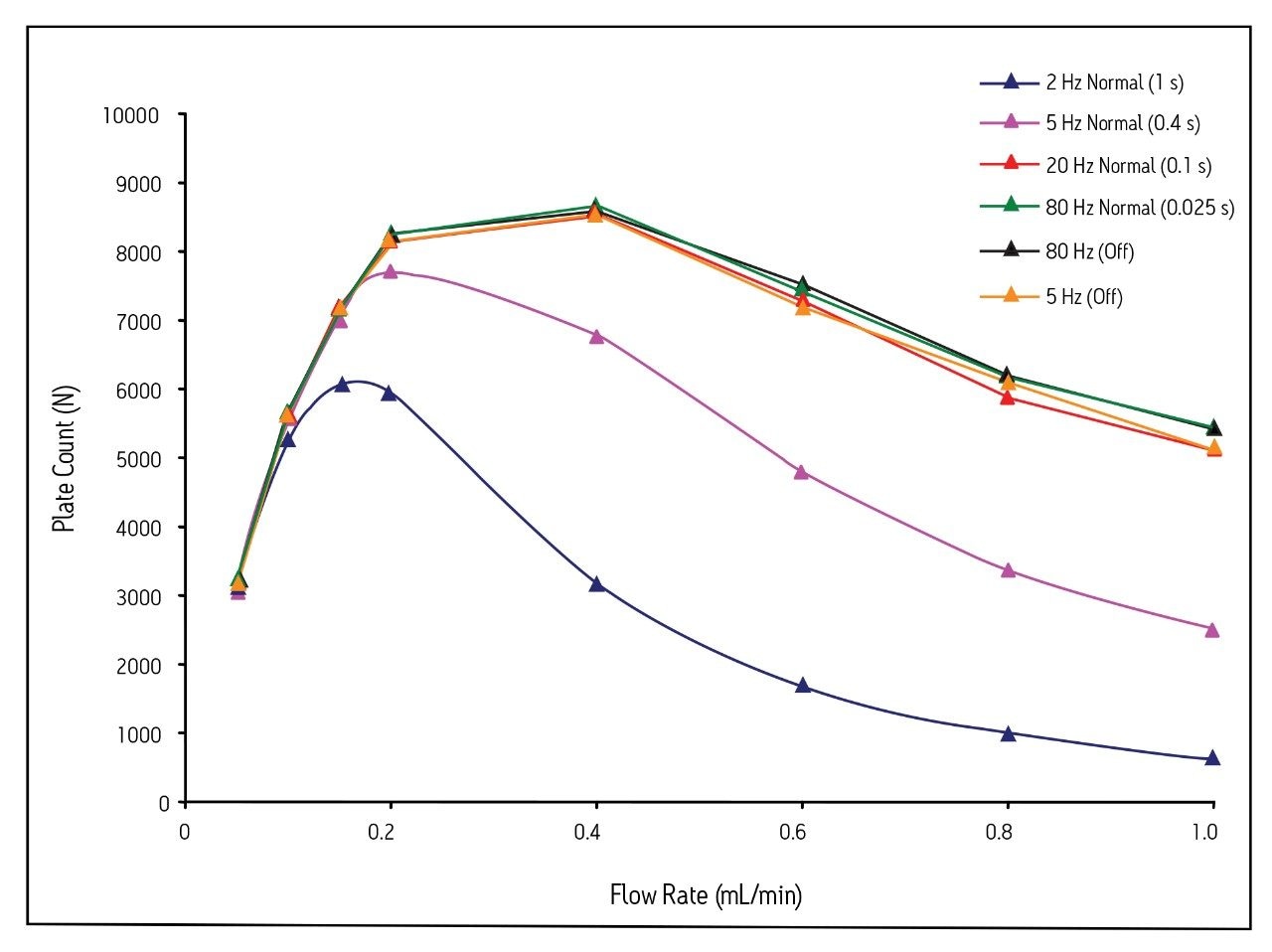
The purpose of this technical note is to show the effect of the detector settings on the measured efficiency of 1.7 μm particle columns. When using UPLC technology for “real-life” applications, it is wise to select the detector data rate that accurately captures the peak shape of the narrowest peak, and then apply a filter time constant that gives optimal signal-to-noise and resolution for the analysis.

Selection of Detector Settings

In order to simplify the selection of the time constant, many detection schemes will combine this setting with the sampling rate. However, this limits the ability for the chromatographer to optimize both resolution and sensitivity. For the plate count measurements performed in this study, we selected a normal time constant, which is equivalent to 2 (1/sampling rate). The plate count was also calculated from data generated using no filter time constant for the 5 and 80 Hz sampling rates for comparison

When constructing van Deemter plots from experimental data, it is important to collect enough data points to capture the true shape of the peak eluting from the column, and ensure that the filter time constant is low enough to avoid peak broadening. This concept is illustrated in Figure 1, in which four different detector settings are compared at two flow rates for acenaphthene. At 0.1 mL/min, the impact of the detector settings is relatively small. The true peak shape and peak width are accurately depicted at a setting as low as 2 Hz (filter time constant = 1 s), and a sufficient number of points is collected across the peak (Table 1). Only an 8% decrease in the plate count was observed compared to a setting of 80 Hz (filter time constant = 0.025 s) at this same flow rate.

The impact of the detector settings is more dramatic at higher flow rates. At 1.0 mL/min, neither the 2 Hz (filter time constant = 1 s) nor the 5 Hz (filter time constant = 0.4 s) setting is adequate to determine the true peak shape (Fig. 1). Therefore, column efficiency (plate count) appears quite low (Table 1). In fact, there is an 8.5- fold improvement in the plate count when a setting of 80 Hz (filter time constant = 0.025 s) instead of 2 Hz (filter time constant = 1 s) is used. These data clearly show that proper detector settings are imperative for accurate determination of a column’s true plate count, especially at high flow rates.

Figure 2 shows the impact of both sampling rate and filter time constant on the plate count across a flow rate range of 0.05–1.0 mL/min. The plate count (N) was calculated using equation 1 below:

where t_R is the retention time of acenaphthene corrected for system retention time and wP is the peak width at 13.4% peak height. Two important pieces of information can be obtained from these data. First, the plate count for a column is strongly impacted by the choice of sampling rate, filter time constant, and flow rate. This is especially true for 1.7 μm particle columns, since they produce extremely narrow peaks. At flow rates above 0.2 mL/min, filter time constants greater than 0.1 s cause significant peak broadening,
and thus do not allow proper calculation of the column efficiency. For practical applications of UPLC technology, performing analysis with a sub-optimal detector sampling rate and filter time constant can result in a loss of resolution and decreased peak height.

For example, at 0.4 mL/min, the plate count for the UPLC column is 3,165 using a setting of 2 Hz (filter time constant = 1 s). The plate count for the same column at the same flow rate using a setting of 80 Hz (filter time constant = off) is 8,600. Since both the chromatographic resolution and peak height have a square root dependence on column efficiency [2], this translates to a 40% loss in resolution and peak height at a setting of 2 Hz (filter time constant = 1 s). Second, the data in Figure 2 show that the plate count for 1.7 μm particle columns is not strongly impacted by filter time constants below 0.1 s. There is less than a 1 % difference in the calculated plate counts for acenapthene when comparing a filter time constant of 0.1 s (20 Hz sampling rate) to no filter time constant (80 Hz sampling rate) at 0.4 mL/min. Even at the highest flow rate tested (1.0 mL/min), the difference between the 0.1 s filter time constant and no filtering is less than 7% (~3 % difference in resolution).

The data in Figure 2 were rearranged to produce van Deemter plots for acenaphthene using different sampling rates and filter time constants (Fig. 3). The HETP (μm) was calculated at each flow rate by dividing the column length by the plate count (N). The linear velocity was calculated by dividing the column length (50 mm) by the system corrected retention time (in seconds) of the void volume marker, thiourea.

As in Fig. 2, the van Deemter curves for the 1.7 μm particle column appear worse at filter time constants above 0.1 s. In addition, the C-terms of the van Deemter curves for the 2 Hz and 5 Hz (filter time constant = normal) settings are much larger than the others. When an upward curvature is observed on such plots, it is always indicative of sub-optimal detector settings.

One of the major benefits of UPLC technology is the ability to use 1.7 μm and 1.8 μm particle columns at high flow rates with minimal compromise in plate count for ultra-high speed separations. If these same columns are used in conjunction with sub-optimal detector settings, this benefit is lost. In addition, the benefits of increased resolution and sensitivity are compromised.

Figure 3 also shows that when a setting of 5 Hz (no filtering) is used, the van Deemter plot overlays with the curves generated using settings of 20 Hz (filter time constant = 0.1 s) and 80 Hz (filter time constant = 0.025 s). This observation is completely expected, and is most noticeable for linear velocities greater than 3 mm/s. Under these circumstances, the C-term is smaller, thus indicating that the column experiences a minimal loss in plate count with increasing flow rate.

To this point, we have only shown plate count and HETP values that have not been corrected for extra-column band spreading. This was done intentionally to show what the average chromatographer would observe for 1.7 μm particle columns. However, it is important to realize that the detector settings themselves, not just the instrument, can be a source of extra-column band spreading. This is illustrated in Figure 4, in which extra-column band spreading (5x the standard deviation of the peak, in μL) is plotted as a function of flow rate, detector sampling rate, and filter time constant.

These data provide evidence that using sub-optimal detector settings contributes heavily to extra-column band spreading, even at low flow rates. At high flow rates, the extra-column band spreading becomes extremely large for the 2 and 5 Hz (filter time constant = normal) settings. This results in low plate counts for 1.7 μm particle columns and van Deemter plots that do not correlate with chromatographic theory (Figs. 2 and 3).

In order to calculate the true efficiency for any LC column, the plate count must be corrected for all sources of extra-column band spreading (volumetric and time-related). This was accomplished using equation 2 below:

where w_CORR is the corrected peak width at 13.4% peak height. This value was obtained using equation 3 below:

where w_SYS is the peak width of an analyte injected with a zero-volume union in place of the LC column.

Using these equations to calculate the corrected plate count at each flow rate, the van Deemter curves shown in Fig. 3 were re-plotted and yielded dramatically different results (Fig. 5). With the exception of the 2 Hz (filter time constant = 1 s) setting, all of the van Deemter curves overlay quite well. This suggests that for detector settings above 5 Hz (filter time constant = 0.4 s), the true plate count for a column can be determined if the data are corrected for extra-column band spreading. However, for many applications of UPLC technology, this correction is not possible, especially for gradient separations. Under these circumstances, the data sampling rate should be optimized using the narrowest peak in the separation, and then a filter time constant that gives optimal signal-to-noise should be applied.

• The measured plate count of a column is strongly impacted by the choice of sampling rate, filter time constant, and flow rate. This is especially true for 1.7 μm particle columns, since they produce extremely narrow peaks
  
• The use of sub-optimal detector settings in conjunction with UPLC technology can lead to losses in resolution and sensitivity
  
• Sub-optimal detector settings contribute heavily to extracolumn band spreading, especially at high linear velocities
  
• Correcting the measured plate count for all sources of extra-column band spreading gives a more accurate determination of the true column performance, independent of the detector settings

1. KM Usher, CR Simmons, JG Dorsey, J. Chromatogr. A 1200 (2008) 122.
   
2. U.D. Neue. HPLC Columns: Theory, Technology, and Practice. New York: Wiley-VCH, 1997.
   
3. KJ Fountain, ES Grumbach, UD Neue, DM Diehl. Waters Technical Note, 720002793EN, 2008.
   
4. L Kirkup, M Foot, M Mullholland, J. Chromatogr. A 1030 (2004) 25.